pcolor(X, Y, C::Matrix{<:Real}; kwargs...)

Creates a colored cells plot using the values in matrix C. The color of each cell depends on the value of each value of C after consulting a color table (cpt). If a color table is not provided via option cmap=xxx we compute a default one.

• X, Y: Vectors or 1 row matrices with the x- and y-coordinates for the vertices. The number of elements of X must match the number of columns in C (is using the grid registration model) or exceed it by one (pixel registration). The same for Y and the number of rows in C. Notice that X and Y do not need to be equispaced.

• X, Y: Matrices with the x- and y-coordinates for the vertices. In this case the if X and Y define an m-by-n grid, then C should be an (m-1)-by-(n-1) matrix, though we also allow it to be m-by-n but we then drop the last row and column from C

• C: A matrix with the values that will be used to color the cells.

• kwargs: This form of pcolor is in fact a wrap up of $plot$ so any option of that module can be used here.

• labels: If this $keyword$ is used then we plot the value of each node in the corresponding cell. Use label=n, where $n$ is integer and represents the number of printed decimals. Any other value like $true$, $"y"$ or $:y$ tells the program to guess the number of decimals.

• font: When label is used one may also control text font settings. Options are a subset of the $text$ attrib option. Namely, the angle and the $font$. Example: $font=(angle=45, font=(5,:red))$. If not specified, it defaults to $font=(font=(6,:black),)$.

D = pcolor(X, Y; kwargs...)

This form, that is without a color matrix, accepts X and Y as before but returns the tiles in a vector of GMTdatasets. Use the kwargs option to pass for example a projection setting (as for example $proj=:geo$).

pcolor(G::GMTgrid; kwargs...)

This form takes a grid (or the file name of one) as input an paints it's cell with a constant color.

• outline: Draw the tile outlines and specify a custom pen if the default pen is not to your liking.

• kwargs: This form of pcolor is a wrap of $grdview$ so any option of that module can be used here. One can for example control the tilling option via $grdview's$ $tiles$ option.

Examples

# Create an example grid
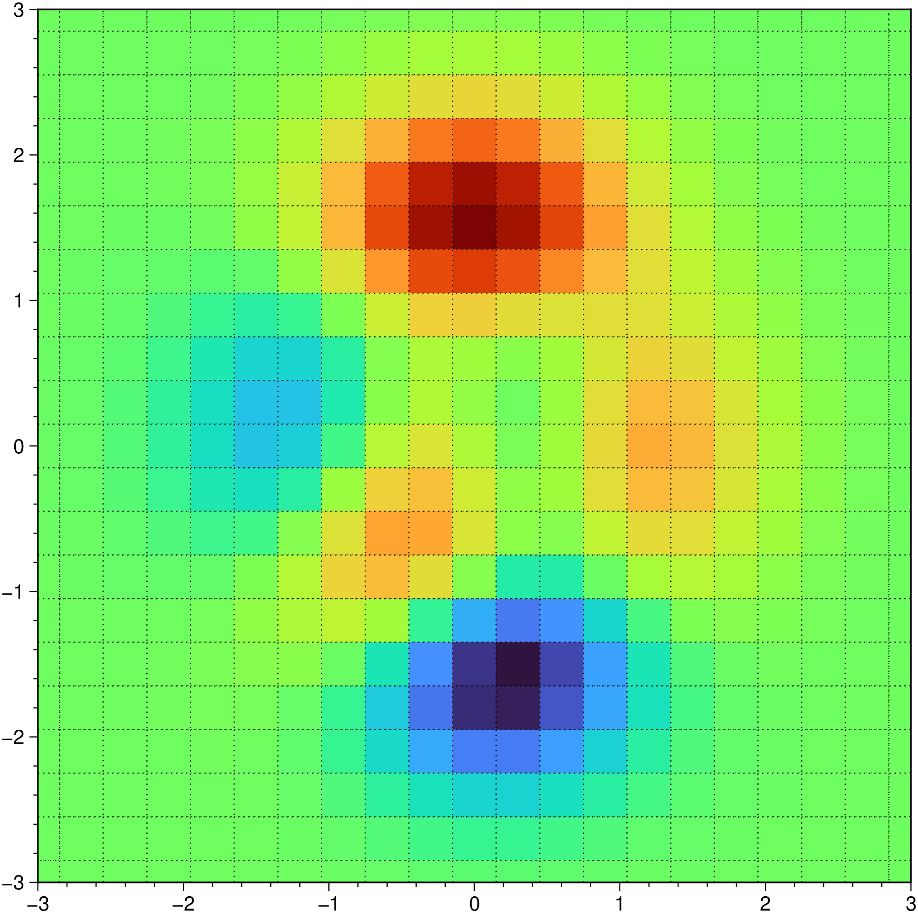
G = GMT.peaks(N=21);

pcolor(G, outline=(0.5,:dot), show=true)

# Now use the G x,y coordinates in the non-regular form
pcolor(G.x, G.y, G.z, show=true)

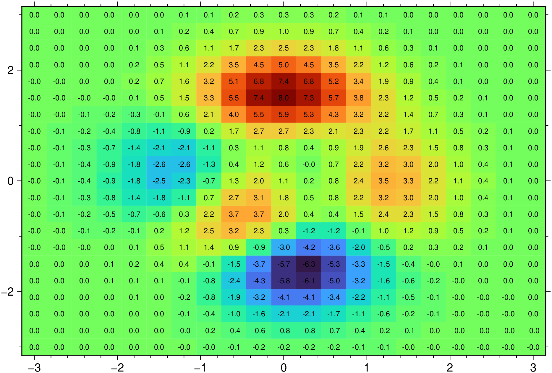
# Add labels to cells using default settings (font size = 6p)
pcolor(G.x, G.y, G.z, labels=:y, show=true)

# Similar to above but now set the number of decimlas in labels as well as it font settings
pcolor(G.x, G.y, G.z, labels=2, font=(angle=45, font=(5,:red)), show=1)

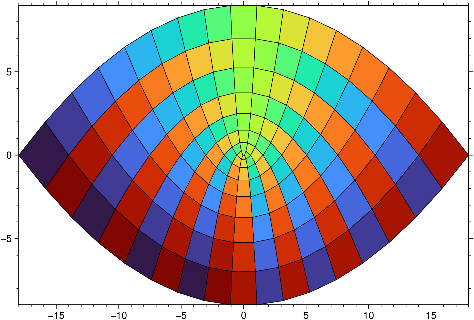
# An irregular grid
X,Y = meshgrid(-3:6/17:3);
XX = 2*X .* Y;	YY = X.^2 .- Y.^2;
pcolor(XX,YY, reshape(repeat([1:18; 18:-1:1], 9,1), size(XX)), lc=:black, show=true)